A/B Testing at Scale: Power, Sequential Testing, and Practical Pitfalls

Author: Ruchita Daga | Faculty: Prof. Jayashree Bagade

Abstract

Online businesses decide what to ship with A/B tests, yet the error rates they quote (5% false positives, 80% power) hold only if the test is planned in advance and analysed once. In practice teams check dashboards daily, stop as soon as the result "looks significant", and track many metrics at once. I simulated a checkout-button experiment (5% baseline conversion, +10% target lift, 2,250 visitors per arm per day) and ran 20,000 synthetic A/A and A/B tests per configuration to measure what these habits cost. Planning required 31,234 visitors per arm (about 14 days); stopping after one week left only 51% power. Checking the p-value every day for 14 days raised the false-positive rate from 5% to 22%, and tracking 10 uncorrected metrics produced at least one false "win" 40% of the time. An O'Brien–Fleming sequential design restored the false-positive rate to 4.8% while keeping 79% power, and reached a decision 3.4 days earlier on average when the effect was real. The lesson: the error rate of an A/B test is a property of the whole decision process, not of the z-test formula.

1. Title and Hook

Imagine Riya, a product analyst at an online store. Her team launches a redesigned checkout button to half of its visitors. She opens the dashboard every morning. On day 2 the p-value reads 0.033: "statistically significant". Her manager is delighted, the new button ships to everyone, and the team moves on.

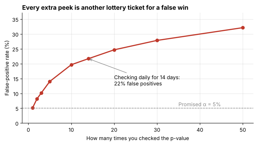
What Riya does not know is that, in the run of my simulation that matches her story, the two buttons were identical. By day 14 the same test would have shown p = 0.65. Nothing improved; the team simply caught random noise at a lucky moment. Repeated across many tests, this habit turns a promised 5% false-alarm rate into roughly 22%: more than one "win" in five is fake. This blog is about how to plan an A/B test so its numbers mean what they claim, and how to look at results early without fooling yourself.

2. Problem and Context

The problem. An A/B test (an online controlled experiment) randomly splits users between the current version (A, the control) and a change (B, the treatment) and compares an outcome such as conversion rate [1]. The classical analysis, a two-proportion z-test, guarantees a 5% false-positive rate only under three conditions: the sample size is fixed in advance, the result is examined once, and one primary hypothesis is tested. Modern experimentation platforms show live results, which makes it very easy to break all three conditions without noticing.

Who faces it. Anyone who decides with experiments: product and growth teams testing features, e-commerce teams testing prices and layouts, marketing teams testing emails and ads, and start-ups with little traffic that are tempted to stop tests early. A systematic review of A/B testing research found it used across web, mobile, e-commerce and many other domains [8].

Why it matters. A false positive ships a change that does nothing, or quietly hurts users, and the team believes it worked. An under-powered test does the opposite: it misses a real improvement and the idea is abandoned. Both waste engineering time and erode trust in data. Practitioners at large experimentation platforms list peeking, low power and multiple testing among the most common mistakes [2][9].

The idea. The fix is not a new statistical test but a disciplined process: decide the smallest effect worth detecting, compute the sample size that gives enough power, and either look once at the end or use a sequential design whose stopping thresholds are built for repeated looks [4][5]. Group sequential methods were developed for clinical trials, where stopping early for benefit or harm is ethically important; the same mathematics applies directly to web experiments [3].

Fixed-horizon versus sequential testing. A fixed-horizon test is simple and has the best power for a given maximum sample size, but you must wait until the end. A sequential test allows early stopping, which saves time when the effect is large, at the cost of slightly stricter thresholds. They are design choices, not rivals: the mistake is running a fixed-horizon test as if it were sequential.

3. Concepts Explained

Null hypothesis and significance level (α). The null hypothesis says A and B have the same true conversion rate. The significance level α is the false-alarm rate we accept: the probability of declaring a difference when none exists (a Type I error). With α = 0.05 and a two-sided test, we reject when |z| > 1.96.

Effect size and minimum detectable effect (MDE). Effect size is the true difference, for example 5.0% → 5.5% conversion: +0.5 percentage points absolute, or +10% relative. The MDE is the smallest effect worth acting on. It is a business decision (what lift pays for the change?), made before the test, not a number read off the results.

Statistical power (1 − β). Power is the probability that the test detects the MDE if it truly exists. The common target is 80%, meaning a 20% chance of missing a real effect (a Type II error). Power grows with sample size and effect size and falls as α becomes stricter.

Sample-size planning. Given the baseline rate, MDE, α and power, a formula (Section 4) gives the number of visitors needed per group. Dividing by daily traffic gives the test duration. Because the effect appears squared in the denominator, halving the MDE roughly quadruples the sample size.

The p-value is not a progress bar. When the null hypothesis is true, the p-value does not slowly converge to "not significant"; it wanders randomly between 0 and 1 as data arrives. Checking it once gives a 5% chance of a false alarm. Checking it many times gives many chances.

Peeking (optional stopping). Peeking means looking at the result repeatedly and stopping the first time p < 0.05. Small example: if two looks were independent, the chance of at least one false alarm would be 1 − 0.95² = 9.75%. Looks on accumulating data are positively correlated, so the real figure is a little lower, and my simulation measured 8.2% for two looks. Either way, it is not 5% [3].

Sequential testing and stopping boundaries. A group sequential design plans K looks in advance and uses a stricter threshold at each look so that the overall false-positive rate stays at α. Pocock's design uses the same threshold at every look [5]. O'Brien–Fleming's design is extremely strict early and close to 1.96 at the end [4]. Alpha-spending functions generalise these to unequal or unplanned look times [6]. Always-valid p-values allow continuous monitoring at any time [3].

Multiple comparisons. Testing many metrics, segments or variants inflates false positives in the same way as peeking. With 10 independent metrics and no real effects, the chance that at least one shows p < 0.05 is 1 − 0.95¹⁰ = 40.1%. The Bonferroni correction tests each at α/m; the Holm step-down procedure controls the same family-wise error with more power [7].

Guardrail metrics. Metrics that must not get worse even if the primary metric improves: page load time, refunds, unsubscribes, errors. They protect users and the business from a "win" that causes harm elsewhere [1].

Statistical versus practical significance. With enough data, even a trivially small difference becomes statistically significant. The decision question is whether the confidence interval for the lift lies above the MDE, not only whether p < 0.05 [2].

4. How It Works

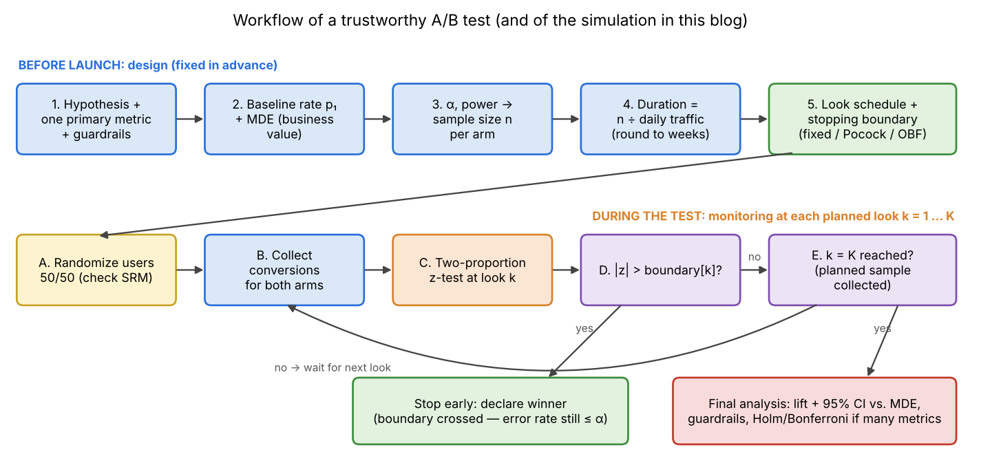
Figure 0. Workflow of a trustworthy A/B test: design is fixed before launch, monitoring happens only at planned looks, and the decision checks practical significance and guardrails.

Workflow.

1. Write the hypothesis, one primary metric and the guardrail metrics.
2. Estimate the baseline rate p₁ from past data and choose the MDE from business value.
3. Choose α and power, and compute the sample size n per arm.
4. Convert n into a duration using daily traffic, and round up to whole weeks.
5. Choose the look schedule (once, or K planned looks) and the stopping boundary (fixed, Pocock or O'Brien–Fleming).
6. Randomize users 50/50 and check the split (sample-ratio mismatch) early.
7. At each planned look, compute the two-proportion z statistic and compare it with that look's boundary; stop only if it is crossed.
8. At the final look, report the lift with a 95% confidence interval, compare it with the MDE, check guardrails, and correct for multiple metrics.

Pseudocode.

## --- design (before launch) ---
n = sample_size(p1=0.05, mde=0.10, alpha=0.05, power=0.80)
K = 14                                     # one look per day
boundary = [c * sqrt(K / k) for k in 1..K] # O'Brien-Fleming, c calibrated

## --- monitoring ---
for k in 1..K:
    collect another n/K users per arm
    z = (rate_B - rate_A) / pooled_standard_error
    if abs(z) > boundary[k]:
        return STOP, "winner" if z > 0 else "loser"
return FINAL_ANALYSIS                      # CI vs MDE, guardrails

A worked trace (from the simulation).

In A/A run #1 of the daily-look simulation, both buttons converted at a true 5.0%. On day 2 (about 4,460 users per arm), the z statistic was about 2.13, so p = 0.033. A naive analyst comparing with 1.96 would stop and ship. Under O'Brien–Fleming the day-2 boundary is 5.56, so the test continues. By day 14 the p-value was 0.65, and the correct conclusion is "no detectable difference".

A small mathematical example: sample size.

The visitors needed per group for two proportions are:

With p₁ = 0.050, p₂ = 0.055, α = 0.05 (z = 1.96) and power 80% (z = 0.84): the first term is 1.96 × √(2 × 0.0525 × 0.9475) = 0.618, the second is 0.84 × √(0.0475 + 0.0520) = 0.265, so n = (0.618 + 0.265)² / 0.005² ≈ 31,234 per group. At 2,250 users per arm per day, that is 13.9 days.

A small mathematical example: the O'Brien–Fleming boundary.

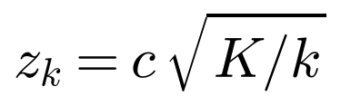
With K = 14 looks and the calibrated c = 2.10: day 1 needs |z| > 2.10 × √14 = 7.86, day 7 needs 2.10 × √2 = 2.97, and day 14 needs 2.10. The final threshold is only slightly stricter than 1.96, which is why little power is lost.

5. Mini-Experiment

Research question. How much do common A/B testing habits (stopping early, checking daily, tracking many metrics) change the real error rates of a test, and do sequential designs and multiple-comparison corrections restore them without losing too much power?

Scenario. An online store tests a redesigned checkout button (B) against the current one (A). The primary metric is checkout conversion.

Dataset. Fully synthetic, generated inside the notebook. Each visitor converts independently with a fixed probability; daily conversion counts per arm are drawn from a binomial distribution using NumPy's random generator with fixed seeds. Synthetic data is used on purpose: because I set the true conversion rates myself, I know the right answer for every simulated test, so false positives and missed effects can be counted exactly. No real customer data is involved.

Table 0. Simulation settings (fixed before running any analysis).

Setting	Value
Baseline conversion (A)	5.0%
Minimum detectable effect	+10% relative (5.0% → 5.5%)
Traffic	2,250 visitors per arm per day
α / power target	0.05 two-sided / 80%
Planned sample	31,234 visitors per arm (≈ 14 days)
Looks tested	1, 2, 3, 5, 10, 14, 20, 30, 50 (equally spaced)
Simulations per configuration	20,000 (40,000 for boundary calibration)
Random seeds	42 (main), 1–7, 11, 100–104 (per experiment, listed in the notebook)

Implementation and environment. Python 3.13, NumPy 2.5, SciPy 1.18, pandas 3.0, statsmodels 0.15 [10], matplotlib 3.11, run as a single Jupyter notebook. The sample-size formula was cross-checked against statsmodels' NormalIndPower (31,234 vs 31,217 per arm; the small gap comes from statsmodels' arcsine effect-size approximation).

Systems compared. (1) Fixed horizon: look once, at day 14, with |z| > 1.96 (the baseline). (2) Naive peeking: look every day, stop the first time |z| > 1.96. (3) Pocock: look every day with one constant, stricter threshold [5]. (4) O'Brien–Fleming (OBF): look every day with a threshold that starts very strict and relaxes to near 1.96 [4]. For multiple metrics: (5) no correction, (6) Bonferroni, (7) Holm [7].

Experiments. (a) Sample size and power curves from the formula. (b) A/A tests (both arms at 5.0%) with 1 to 50 looks: every "winner" is a false positive. (c) Calibrating Pocock and OBF constants by bisection so that the simulated A/A false-positive rate is 5% for 14 looks, then evaluating them on fresh simulations. (d) A/B tests with a true +10% lift to measure power and time to decision. (e) An ablation over true lift from 0% to +20%. (f) Ten unrelated metrics with no real effect. (g) A very large test with a tiny true lift (+1%) to separate statistical from practical significance.

Evaluation methodology (defined before results).

Metric	Definition
False-positive rate	Share of A/A simulations in which the method declared a winner at any look. Target: ≤ 5%.
Power	Share of A/B simulations (true +10% lift) in which the method declared B the winner. Target: ≥ 80%.
Average days to decision	Mean look at which the test stopped; tests that never crossed a boundary count as 14 days.
Stopped by day 7	Share of simulations that declared B the winner within the first week.
Family-wise error rate	Share of simulations with at least one false "win" among 10 metrics.
Monte Carlo error	95% uncertainty of a simulated rate: ±1.96√(r(1−r)/N). With N = 20,000 it is ±0.3 points at 5% and ±0.6 points at 80%.

Calibration and evaluation use different random seeds, so the boundaries are never judged on the same simulations they were tuned on.

6. Results

All numbers below are read from the executed notebook ab_testing_at_scale.ipynb and its exported results_*.csv files.

6.1 Planning: sample size and power

Table 1. Visitors needed per arm for different MDEs (baseline 5%, α = 0.05, power 80%).

Relative MDE	Absolute lift (pp)	n per arm	Total visitors	Days at 2,250/arm/day
2%	0.10	752,703	1,505,406	334.5
5%	0.25	122,124	244,248	54.3
10%	0.50	31,234	62,468	13.9
15%	0.75	14,193	28,386	6.3
20%	1.00	8,158	16,316	3.6
30%	1.50	3,780	7,560	1.7

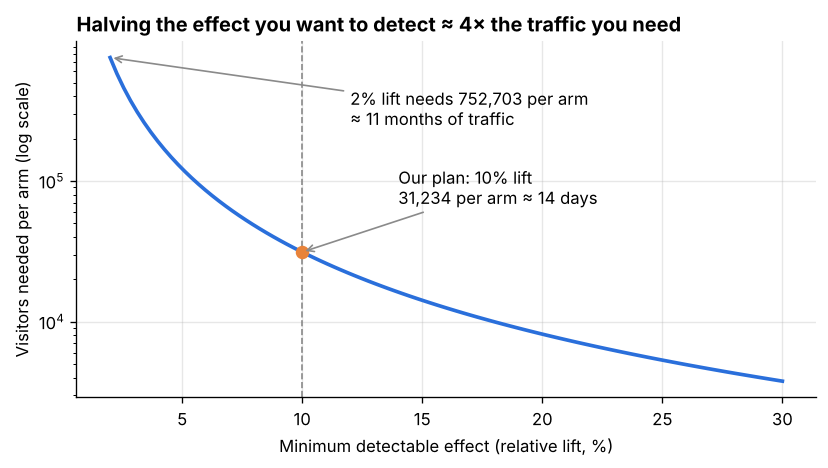
Figure 1. Required sample size per arm versus MDE (log scale). Halving the MDE roughly quadruples the traffic needed.

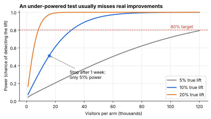
Figure 2. Power versus sample size for three true lifts. Stopping the 10%-lift test after one week (15,750 per arm) gives only 51% power.

6.2 The cost of peeking

Table 2. False-positive rate of naive peeking in 20,000 A/A tests (no real difference).

Number of looks	False-positive rate	vs. promised 5%
1	5.2%	1.0×
2	8.2%	1.6×
3	10.1%	2.0×
5	14.0%	2.8×
10	19.7%	3.9×
14 (daily)	21.7%	4.3×
20	24.7%	4.9×
30	27.9%	5.6×
50	32.1%	6.4×

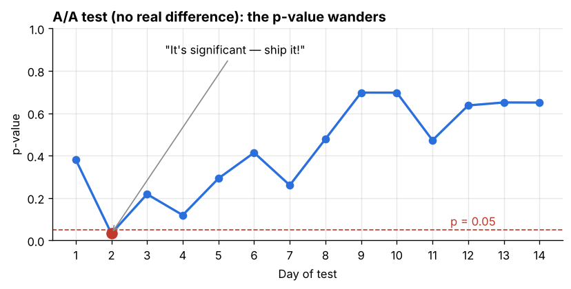
Figure 3. One A/A run checked daily: the p-value dips to 0.033 on day 2 and ends at 0.65 on day 14.

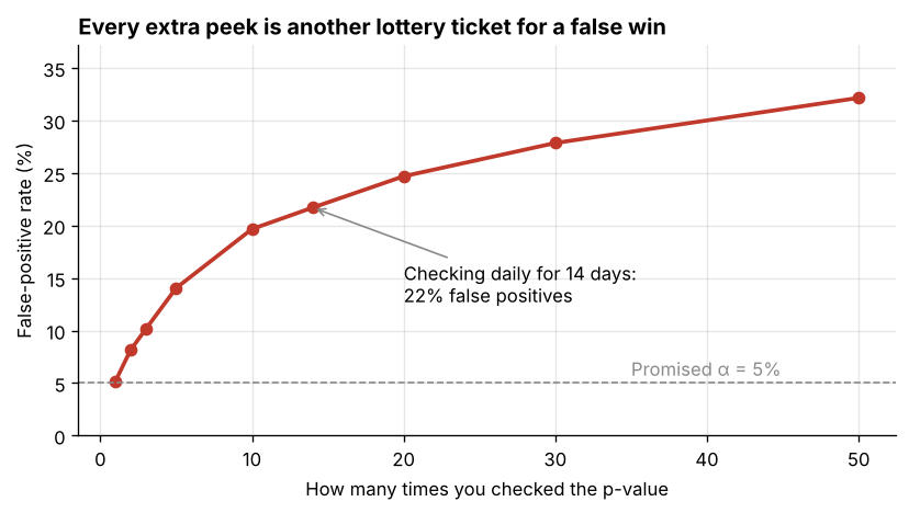
Figure 4. False-positive rate of naive peeking versus number of looks (20,000 A/A simulations per point).

6.3 Sequential boundaries

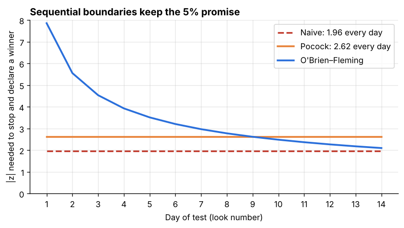
Figure 5. Stopping boundaries for 14 daily looks: naive 1.96, Pocock 2.62 at every look, and O'Brien–Fleming from 7.86 on day 1 to 2.10 on day 14.

Table 3. Error rates and speed of each method for 14 daily looks (20,000 fresh simulations each).

Method	False-positive rate (A/A)	Power (true +10%)	Avg. days to decision
Fixed horizon (look once on day 14)	4.5%	80.6%	14.0
Naive daily peeking at 1.96	21.5%	87.7%	6.6
Pocock (|z| > 2.62 every day)	4.8%	67.4%	9.6
O'Brien–Fleming (7.86 → 2.10)	4.8%	79.1%	10.6

6.4 Ablation: how the true effect size changes the picture

Table 4. Fixed horizon vs. O'Brien–Fleming across true lifts (14 looks, 20,000 simulations per row; at +0% the "winner" rate is the false-positive rate).

True lift	Fixed: declares B winner	OBF: declares B winner	OBF: avg. days to decision	OBF: stopped by day 7
+0%	4.7%	4.8%	13.9	0.3%
+5%	29.2%	28.1%	13.1	2.8%
+10%	80.0%	78.3%	10.6	16.7%
+15%	98.6%	98.4%	7.9	49.7%
+20%	100.0%	100.0%	6.1	82.5%

6.5 Multiple metrics

Table 5. Chance of at least one false "win" among 10 metrics with no real effect (20,000 simulations; Holm on 5,000).

Rule	P(at least one false win)
No correction (p < 0.05 each)	40.0% (theory 40.1%)
Bonferroni (p < 0.005 each)	4.7%
Holm step-down	5.3%

6.6 Statistical versus practical significance

In one very large simulated test (2,000,000 users per arm, true lift +1% relative), the observed lift was +0.087 percentage points with 95% CI [0.044, 0.130] and p = 0.0001. The result is highly significant, yet the entire interval lies far below the 0.5-point MDE the business said was worth shipping.

What the numbers show.

• Planning decides what a test can find. At 2,250 users per arm per day, only lifts of about 10% or more are detectable in two weeks. A 2% lift would take 11 months (Table 1). Teams with modest traffic should test bolder changes rather than run weaker tests.
• Stopping early mostly hides real wins. Stopping the 10%-lift test after one week gives 51% power (Figure 2): a coin flip on noticing a real improvement. A "no difference" result from an under-powered test is weak evidence, not proof of no effect.
• Peeking inflates false positives steadily. Each extra look is another chance for noise to cross 1.96: 8.2% for 2 looks, 21.7% for 14 daily looks, 32.1% for 50 (Table 2, Figure 4). The single run in Figure 3 shows how convincing a false win can look on the day it happens.
• Naive peeking only looks more powerful. Its 87.7% power in Table 3 is bought with a 21.5% false-positive rate; it is not a fair comparison.
• O'Brien–Fleming is the best compromise here. It keeps the false-positive rate at 4.8%, loses only about 1.5 points of power against the fixed design (79.1% vs 80.6%, close to Monte Carlo error), and decides 3.4 days earlier on average. Pocock stops even earlier (9.6 days) but loses 13 points of power, because its constant 2.62 threshold is also applied at the final look.
• Early stopping pays off most for big effects. With a +20% true lift, OBF stopped by day 7 in 82.5% of tests and took 6.1 days on average; with a +5% lift it almost never stopped early (Table 4). Sequential designs save time exactly when the change is clearly good, which is when waiting is most costly.
• Many metrics behave like many peeks. Ten uncorrected metrics gave a 40% chance of a false win; Bonferroni and Holm brought it back to about 5% (Table 5).
• Significance is not importance. Section 6.6 shows a p-value of 0.0001 for a lift too small to matter. Decisions should compare the confidence interval with the MDE.

6.7 Trade-offs observed

Sequential designs add planning work (choosing K and calibrating boundaries) and slightly stricter final thresholds (2.10 instead of 1.96 for OBF), which costs a little power. In exchange they make early looks safe. Bonferroni is simple but conservative when metrics are correlated; Holm is never less powerful and is just as easy to compute. The two OBF power figures (79.1% in Table 3 and 78.3% in Table 4) come from different random seeds and differ by about the Monte Carlo error of ±0.6 points.

7. Limitations and Responsible Use

Scope and statistics. These are simulations of one scenario (5% baseline, +10% MDE, 14 looks). The qualitative lessons are well established in the literature [1][3][4], but the exact percentages depend on these settings. Each simulated rate carries Monte Carlo error of about ±0.3 to ±0.6 percentage points, so differences smaller than about 1 point should not be over-interpreted.

Synthetic data is cleaner than reality. Real traffic has weekday and weekend cycles, holidays, bots, returning visitors, and novelty or primacy effects (users react to change itself). Real tests should run for whole weeks even if the planned sample is reached sooner, and should be checked for outliers and bot traffic.

Independence assumption. The simulation treats every visitor as independent. In practice one user may visit many times. Randomization should be by user, and the analysis must use the same unit as the randomization; otherwise standard errors are too small and false positives rise.

Normal approximation. The z-test relies on large counts, which holds here (hundreds of conversions per arm per day). With very low conversion rates or small samples, exact tests or bootstrap methods are safer.

Equally spaced looks. The boundaries assume K equal looks. Real daily traffic varies. Production systems use alpha-spending functions [6] or always-valid p-values [3] that adapt to the actual share of data collected.

Sample-ratio mismatch. If the split between A and B is far from 50/50, randomization or logging is broken and no statistical method can rescue the result. This check should run early in every test.

Ethics and user impact. Experiments change what real people see and sometimes what they pay. Guardrail metrics (refunds, complaints, page speed) should be monitored, and tests should stop early for clear harm, not only for wins. Dark patterns and changes that mislead users should not be tested at all.

Privacy. An A/B test needs only assignment and outcome events. Collect the minimum, aggregate where possible, and follow consent rules for tracking.

From simulation to a real platform. A production setup would add automated SRM checks, pre-registered metrics, alpha-spending or always-valid inference, variance reduction, and a review step before shipping.

8. Practical Recommendations

When A/B testing is useful: the change can be randomized per user; there is enough traffic to detect the smallest lift worth acting on within a few weeks; the outcome can be measured reliably and soon after exposure.

When it may be unnecessary or unsuitable: traffic is so low that only huge effects are detectable (use qualitative research or bolder changes instead); the change is required anyway (a bug fix, a legal requirement); or users influence each other (social or marketplace features), where simple randomization breaks and cluster designs are needed.

How to run a trustworthy test:

1. Write down one primary metric and the guardrail metrics before launch.
2. Choose the MDE from business value, then compute the sample size and test duration (Section 4). Round up to whole weeks.
3. Decide the look schedule in advance. If anyone will check results early, use a sequential design: O'Brien–Fleming if power matters most, Pocock only if very early stopping is the priority [4][5].
4. Never stop a fixed-horizon test because the dashboard "looks significant".
5. With several metrics or variants, apply Holm (or Bonferroni) to the confirmatory ones; treat the rest as exploratory [7].
6. Check the 50/50 split (sample-ratio mismatch) on day 1.
7. Report the lift with a 95% confidence interval and compare it with the MDE, not only the p-value.
8. Run an A/A test on your own platform. If it "finds" winners more than about 5% of the time, the pipeline or the process is broken [1].

9. References and Reproducibility

References

[1] Kohavi, R., Tang, D., Xu, Y. (2020). Trustworthy Online Controlled Experiments: A Practical Guide to A/B Testing. Cambridge University Press.

https://doi.org/10.1017/9781108653985

[2] Kohavi, R., Deng, A., Vermeer, L. (2022). A/B Testing Intuition Busters: Common Misunderstandings in Online Controlled Experiments. KDD 2022.

https://www.lukasvermeer.nl/publications/paper/2022/08/14/ab-testing-intuition-busters-common-misunderstandings.html

[3] Johari, R., Pekelis, L., Walsh, D. J. (2019). Always Valid Inference: Bringing Sequential Analysis to A/B Testing. arXiv:1512.04922.

https://arxiv.org/abs/1512.04922

[4] O'Brien, P. C., Fleming, T. R. (1979). A Multiple Testing Procedure for Clinical Trials. Biometrics, 35(3), 549–556.

https://doi.org/10.2307/2530245

[5] Pocock, S. J. (1977). Group Sequential Methods in the Design and Analysis of Clinical Trials. Biometrika, 64(2), 191–199.

https://doi.org/10.1093/biomet/64.2.191

[6] Lan, K. K. G., DeMets, D. L. (1983). Discrete Sequential Boundaries for Clinical Trials. Biometrika, 70(3), 659–663.

https://www.jstor.org/stable/2336502

[7] Holm, S. (1979). A Simple Sequentially Rejective Multiple Test Procedure. Scandinavian Journal of Statistics, 6(2), 65–70.

https://www.jstor.org/stable/4615733

[8] Quin, F., Weyns, D., Galster, M., Silva, C. C. (2023). A/B Testing: A Systematic Literature Review. arXiv:2308.04929.

https://arxiv.org/abs/2308.04929

[9] GrowthBook documentation. Experimentation Problems (peeking, multiple testing).

https://docs.growthbook.io/using/experimentation-problems

[10] statsmodels documentation. Power and sample size calculations (statsmodels.stats.power).

https://www.statsmodels.org/

Reproducibility

Everything in this blog comes from one Jupyter notebook, ab_testing_at_scale.ipynb, plus diagram.py for Figure 0. The data is synthetic and generated inside the notebook with fixed random seeds, so re-running it reproduces every table and figure exactly. Result tables are exported as results_sample_size.csv, results_peeking.csv, results_sequential.csv, results_ablation_effect_size.csv and results_multiple_comparisons.csv. Code and outputs: https://github.com/RuchitaDaga/ab-testing-at-scale.

Conclusion

An A/B test is only as trustworthy as the process around it. In my simulation, the same z-test formula produced a 5% false-positive rate when used as designed and 22% when checked daily, and an under-powered one-week test missed a real 10% improvement about half the time. None of these failures would show up in a single "p < 0.05" headline. The fixes are cheap: plan the sample size from a business-driven MDE, decide in advance when you will look, use sequential boundaries such as O'Brien–Fleming if you must look early, correct for multiple metrics, and judge results by confidence intervals against the MDE. A natural next step is to repeat this analysis on real experiment logs with day-of-week effects and returning users, where alpha-spending and always-valid methods become essential.